Probability Audit (free Excel tool)

There’s a link to the free model at the bottom of the article

Contents

• The motivation
• The model
• The mathematics
• Link to the tool

Motivation

• I am a credit risk manager. At the start of the year, I have assessed the probabilities of my debtors defaulting in the course of the year (which I am rather naively assuming to be independent). At the end of the year, I have a list of those who have defaulted and those who have not and I would like to evaluate how good my probability assessments were, on average.
• I am a portfolio manager in an oil and gas exploration company. At the start of the year, my subsurface teams have assessed the probabilities that the exploration wells I drill during the year will discover oil. At the end of the year, I have a list of those that discovered oil and those that did not and I would like to evaluate how good my probability assessments were, on average.
• I am testing myself at assessing probabilities, so I have taken a calibration test where I have answered a list of questions and provided a probability that my answer to that question is correct. I would like to see whether, on average, I over- or under-estimate probability

The model

We have a sequence of probabilities, each of which describes our belief in the likelihood that a given event will take place (default, discovery, etc.). The events are binary, so they either happen or they don’t.

For reasons explained here, it’s very difficult to say anything about individual assessments on the basis of a single outcome, so we look at the outcome of the whole sequence to try and reduce the uncertainty.

The simplest way to do this is to look at the total number of events that took place. How many debtors defaulted; how many discoveries were drilled?

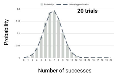
We calculate the probability distribution for the number of defaults, discoveries, whatever is the event outcome we’re counting. The distribution will look something like this.

By looking at the actual number compared to this distribution, we can see whether we over- or underestimate probabilities.

There are a number of ways of calculating or approximating this distribution

1. You can hit it with a Monte Carlo sledge hammer
2. You can calculate the probabilities directly
3. You can use the Central limit theorem and approximate the distribution with a Normal distribution.

Direct calculation

We call the outcomes that we count successes . This makes sense for oil discoveries, but is frankly a little odd for credit defaults. Nonetheless.

If you have just one event with some probability of success, say 20%, then after that event, the probability of your count being 1 is 20% and it being 0 is 80%.

Say the next event has probability 30%. Then the probability of the count being zero is the probability the count after the first was zero (80%) times the probability the second also fails, i.e. 80% x 70%.

There are two ways having a count of 1 after 2 events. Event 1 failed (80%) and event 2 was a success (30%) and vice versa, with probabilities 20% and 70%. The probability of a count of one is then 80% x 30% + 20% x 70%.

To have a count of two, we had to have success in both events.

Now, continuing in this vein seems pretty tedious, but there’s a pattern. There are two ways of getting a given number of outcomes on a given round. Either there was one fewer on the previous round and the current round was a success or there were the same number on the previous round and the current round was a failure. We just have to multiply the probabilities of these two cases in the previous round with the corresponding probabilities in the current round and add them together. This is implemented in the spreadsheet to which there is a link at the bottom of the page.

Note, including dependencies here doesn’t change the basic mathematics — it’s just a question of book-keeping.

Central limit theorem

If we think of each event as a random variable that takes a value 1 or 0 then the count is just the number we get adding all these random variables together.

The central limit theorem tells is that if we add enough random variables together the distribution of the result tends to a normal distribution whose mean is the sum of the means of all the constituent variables and whose variance is the sum of the variances (if they are independent). This is also implemented in the spreadsheet.

Including dependence here is a bit trickier because you have to calculate covariances to get the variance of the sum right.

The math

The tool

You can find a copy of the spreadsheet tool here.

It is set up for sequence lengths up to 20, but once you have a sense of the logic, it’s a simple matter to copy cells down and across to extend the direct method.